Can MMM Measure How Channels Work Together?
Moving from channel-level contribution reporting towards explicit cross-channel measurement
This post started with a question from a colleague: when we report the contribution of each marketing channel, are we actually measuring how those channels work together, or are we still largely evaluating them one at a time?
The question has stayed with me because most campaigns are planned as systems whose parts are meant to support one another, yet the measurement usually collapses into a familiar table with one row per channel, a contribution figure and a return on ad spend (ROAS). We plan jointly but continue to report largely channel by channel.
Traditional marketing mix modelling (MMM) is not wrong, and additive contribution reporting remains useful, well understood and often exactly what a stakeholder needs. The more specific question explored here is whether we can represent and report the interaction between channels explicitly, rather than leaving it unparameterised and potentially conflated with channel main effects or other correlated drivers.
What does the existing research say?
Estimating synergy or interaction between marketing activities has an established research history, so this post builds on an existing tradition rather than presenting the idea as new. The table below summarises the work I lean on.
| Study | What it shows | Why it matters here |
|---|---|---|
| Naik & Raman (2003) (Naik and Raman 2003) | Extends a dynamic advertising model to estimate direct media effects and synergy between television and print. | Establishes that multimedia synergy can be explicitly parameterised and estimated. |
| Naik, Raman & Winer (2005) (Naik et al. 2005) | Advertising and promotion can amplify or attenuate one another, making marketing-mix planning a joint decision. | Supports allowing both positive and negative interactions and considering allocation jointly. |
| Naik & Peters (2009) (Naik and Peters 2009) | Uses a hierarchical structure for within-media, cross-media and higher-order synergies across online and offline channels. | Provides a precedent for imposing structure when several interactions are considered. |
| Kireyev, Pauwels & Gupta (2016) (Kireyev et al. 2016) | In a banking application, display advertising is estimated to affect paid-search conversion, costs, returns and optimal allocation. | Provides an applied example of a plausible directional relationship between two channels. |
| Jin et al. (2017) (Jin et al. 2017) | In smaller datasets, priors can materially affect posterior estimates, and parameter uncertainty carries into media optimisation. | Shows that estimation is already demanding before interaction parameters are added. |
| Sun et al. (2017) (Sun et al. 2017) | Geo-level hierarchical modelling can provide more observations, more useful spend variation and tighter credible intervals than national-only modelling. | Shows how cross-sectional variation and partial pooling can improve estimation when one aggregate time series is weak. |
Although estimating synergy is well established, the model developed here extends that idea by allowing the effect of channel \(j\) on channel \(i\) to differ from the reverse relationship. This directional treatment is my proposed extension and is kept separate from the empirical findings of the papers above.
Proposed directional interaction model
Start with the conventional additive media component. Writing \(m_{i,t}\) for the transformed activity of channel \(i\) at time \(t\) (spend after carryover and saturation), a standard MMM adds the channels up:
\[ C_t = \sum_{i=1}^{N} \beta_i\, m_{i,t}. \]
This is interpretable and decomposes cleanly, but \(\beta_i\) is a property of channel \(i\) alone, with no mechanism through which one channel can change the effectiveness of another. Cross-channel effects do not vanish in an additive model simply because they are not represented explicitly; an omitted interaction may instead be:
- aliased with the channel main effects;
- attributed to correlated regressors;
- left as residual structure the model does not capture;
- associated with poorer out-of-sample prediction;
- absorbed into wider posterior uncertainty.
None of these outcomes means that the baseline or controls have reliably absorbed the interaction. We can represent it explicitly by keeping the additive backbone and multiplying each channel’s contribution by a term that depends on the other channels. For channel \(i\):
\[ C_{i,t}^{\mathrm{mix}} = \underbrace{\beta_i\, m_{i,t}}_{\text{reference}}\, \exp\!\left( \sum_{j \neq i} \gamma_{ij}\, m_{j,t} \right), \]
which sits inside the wider outcome model
\[ y_t = \alpha + \sum_{i=1}^{N} C_{i,t}^{\mathrm{mix}} + \mathbf{x}_t^{\top}\boldsymbol{\delta} + \varepsilon_t, \]
where \(\mathbf{x}_t\) carries the non-media drivers such as controls, trend, seasonality and holidays, while the exponential keeps the multiplier positive so that a channel’s contribution can scale up or down without flipping sign.
What the parameters mean
The interpretation of every parameter depends on the scale of the transformed media. Raw spend is max-scaled into \([0,1]\), then geometric adstock is applied without renormalisation and passed through a \(\tanh\) saturation, which bounds each channel’s transformed media \(m_{i,t}\) at roughly \(b_i \approx 1\). The resulting \(m_{i,t}\) lies in approximately \([0, b_i]\), close to but not exactly \([0,1]\), and reaches its channel maximum only under sustained heavy spend.
- Base effectiveness, \(\beta_i\). If the transformed media output is normalised to approximately \([0,1]\), then \(\beta_i = 0.10\) represents a reference contribution of up to roughly 10% of average sales at that channel’s maximum transformed activity, rather than a ROAS.
- Directional interaction, \(\gamma_{ij}\). This is the effect of modifier channel \(j\) on the effectiveness of channel \(i\), acting as a log-multiplier. When channel \(j\) is near its maximum transformed activity (\(m_{j,t}\approx 1\)), it scales channel \(i\)’s effectiveness by about \(e^{\gamma_{ij}}\). For example, \(\gamma_{ij}=0.50\) implies roughly a \(e^{0.50}-1\approx 65\%\) lift at that level, while a negative \(\gamma_{ij}\) implies suppression and \(\gamma_{ij}\) need not equal \(\gamma_{ji}\).
This gives three quantities worth naming, defined draw by draw:
\[ C_{i,t}^{\mathrm{ref}} = \beta_i\, m_{i,t}, \qquad M_{i,t} = \exp\!\left(\sum_{j\neq i}\gamma_{ij}\, m_{j,t}\right), \qquad C_{i,t}^{\mathrm{mix}} = C_{i,t}^{\mathrm{ref}}\, M_{i,t}, \]
\[ C_{i,t}^{\mathrm{int}} = C_{i,t}^{\mathrm{mix}} - C_{i,t}^{\mathrm{ref}}. \]
The reference contribution \(C^{\mathrm{ref}}\) is obtained by setting the interaction multiplier to one, making it a model-derived reference rather than an experimentally identified estimate of what the channel would have generated if every other channel had been switched off. The realised-mix contribution \(C^{\mathrm{mix}}\) is the inferred contribution under the surrounding media environment that actually occurred. Their difference is the interaction increment \(C^{\mathrm{int}}\), which is positive when other channels amplify the channel and negative when they suppress it. This increment belongs to the existing channels and should not be treated as a spendable extra channel. I sometimes use “silo contribution” as shorthand for \(C^{\mathrm{ref}}\), but it is only a nickname for the multiplier-off reference.
Direction matters
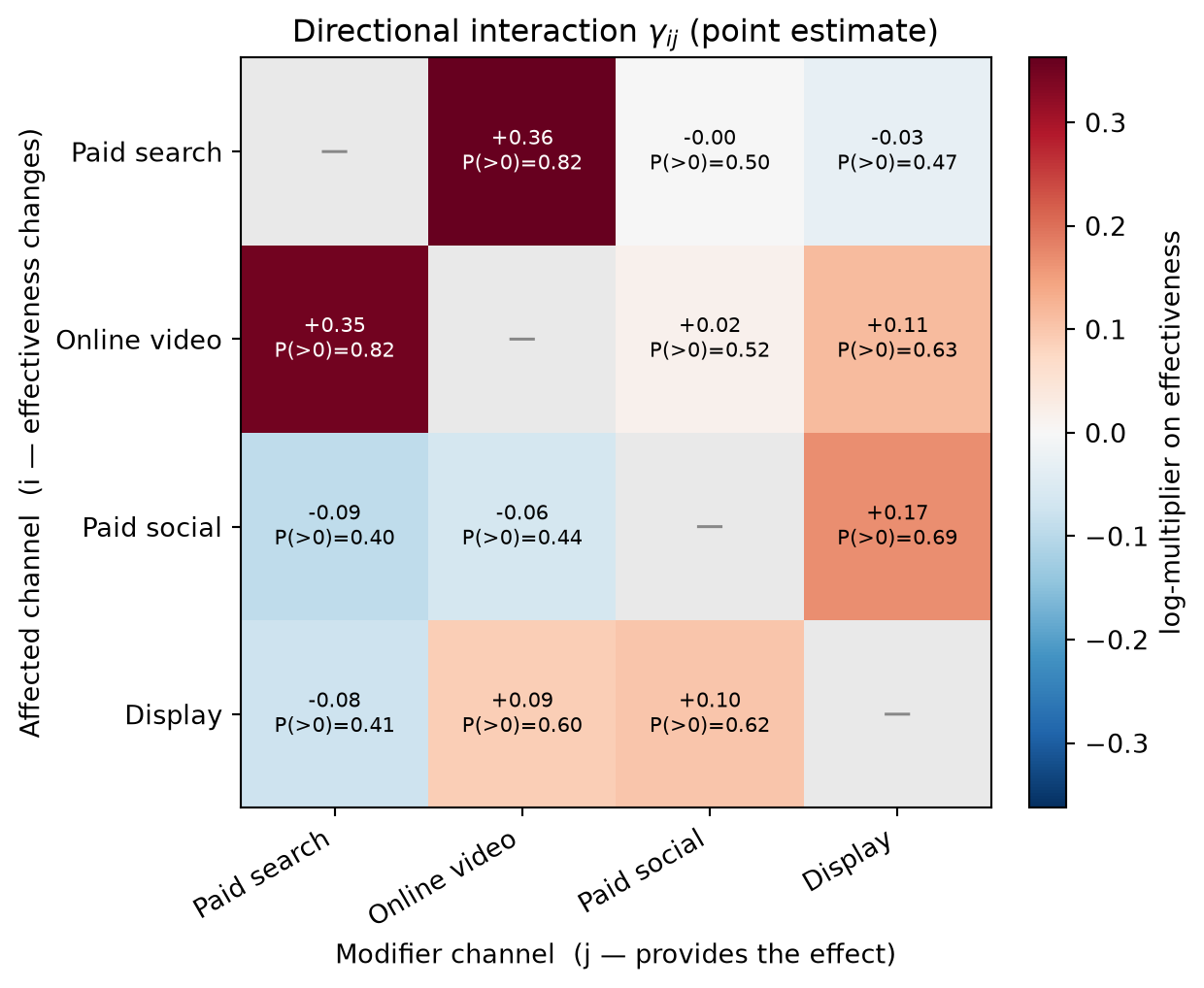
The interaction is directional, and that is the point. Video may modify paid-search effectiveness without paid search returning the favour, so in general \(\gamma_{\text{search,video}} \neq \gamma_{\text{video,search}}\). The figure below shows an example output matrix: rows are the affected channel \(i\); columns are the modifier channel \(j\); the diagonal is masked because a channel does not modify itself. Each cell also gives the posterior probability the effect is positive.
The clearest signal is online video amplifying paid search (top row); the other directions sit close to zero.
Why interactions are applied after adstock and saturation
The interaction term acts on transformed media \(m_{j,t}\), not raw spend, so the modelling sequence is:
\[ \text{spend} \rightarrow \text{adstock (carryover)} \rightarrow \text{saturation (diminishing returns)} \rightarrow \text{interaction layer} \rightarrow \text{contribution} \]
Applying the interaction after saturation limits how quickly additional spend can change the multiplier. As a channel moves further into saturation, further spend produces progressively smaller changes in both its transformed exposure and its effect on other channels. This does not remove the need to control the scale of the interaction coefficients: bounded transformed media helps control the input to the multiplier, but the exponential can still become large, and the prior on \(\gamma\), the media scaling and the number of simultaneously active modifiers all matter. Placing the interaction before the transforms, or on raw spend, would encode different assumptions; tying it to effective media simply keeps the input bounded and the interpretation on the effectiveness scale.
Building the model in PyMC
Building the model directly in PyMC makes the interaction structure, dimensions and derived quantities explicit, rather than requiring the specification to fit within the assumptions of a pre-built MMM class.
Show the PyMC model code
import numpy as np
import pymc as pm
import pytensor.tensor as pt
from pymc_extras.prior import Prior
from pymc_marketing.mmm import GeometricAdstock, TanhSaturation

# Off-diagonal directional pairs: aff_idx = affected channel i, mod_idx = modifier j.
# One free gamma per directional pair; no diagonal parameters are created, so
# nothing disconnected from the likelihood is sampled.
off = ~np.eye(n_channels, dtype=bool)
aff_idx, mod_idx = np.where(off)                                  # length N(N-1)
pair_labels = [f"{names[j]}->{names[i]}" for i, j in zip(aff_idx, mod_idx)]

coords = {
    "date": dates,
    "channel": channel_names,           # affected channel i
    "modifier_channel": channel_names,  # modifier channel j
    "interaction": pair_labels,         # one entry per directional pair
    "control": control_names,
}

with pm.Model(coords=coords) as model:
    # --- Data containers ---
    media = pm.Data("media", media_scaled, dims=("date", "channel"))          # max-scaled spend in [0, 1]
    controls = pm.Data("controls", controls_scaled, dims=("date", "control"))

    # --- Priors ---
    intercept = Prior("Normal", mu=0.8, sigma=0.15).create_variable("intercept")
    beta = Prior("HalfNormal", sigma=0.15, dims="channel").create_variable("beta")   # base effectiveness >= 0
    gamma_offdiag = Prior("Normal", mu=0.0, sigma=0.40,
                          dims="interaction").create_variable("gamma_offdiag")       # one per directional pair
    sigma = Prior("HalfNormal", sigma=0.03).create_variable("sigma")

    # Scatter the off-diagonal parameters into a matrix; the diagonal stays zero.
    gamma_full = pt.set_subtensor(pt.zeros((n_channels, n_channels))[aff_idx, mod_idx], gamma_offdiag)
    gamma_eff = pm.Deterministic("gamma_eff", gamma_full, dims=("channel", "modifier_channel"))

    # --- Adstock + saturation (tight, pre-calibrated priors) ---
    adstock = GeometricAdstock(l_max=12, normalize=False, priors={
        "alpha": Prior("TruncatedNormal", mu=alpha_cal, sigma=0.05, lower=0, upper=1, dims="channel")})
    saturation = TanhSaturation(priors={
        "b": Prior("TruncatedNormal", mu=b_cal, sigma=0.05, lower=0, dims="channel"),
        "c": Prior("TruncatedNormal", mu=c_cal, sigma=0.05, lower=0, dims="channel")})
    m = saturation.apply(adstock.apply(media))                    # transformed media m_{i,t}

    # --- Contribution decomposition (all tracked as deterministics) ---
    reference = pm.Deterministic("reference_contribution_scaled",
                                 m * beta, dims=("date", "channel"))            # beta_i * m_{i,t}
    log_multiplier = pt.dot(m, gamma_eff.T)                       # sum_j gamma_ij * m_{j,t}
    multiplier = pm.Deterministic("interaction_multiplier",
                                  pt.exp(log_multiplier), dims=("date", "channel"))
    realised_mix = pm.Deterministic("realised_mix_contribution_scaled",
                                    reference * multiplier, dims=("date", "channel"))

    # --- Expected sales + likelihood ---
    control_effect = pt.dot(controls, Prior("Normal", 0, 0.10, dims="control")
                            .create_variable("control_beta"))
    # (yearly Fourier seasonality and holiday events omitted here for brevity)
    mu = intercept + realised_mix.sum(axis=-1) + control_effect + seasonality + holidays
    pm.Normal("y", mu=mu, sigma=sigma, observed=y_scaled, dims="date")
The interaction is well-defined because the channel / modifier_channel dimensions pin down the direction of \(\gamma_{ij}\), while the interaction dimension holds exactly one parameter per directional off-diagonal pair. Filling the diagonal deterministically with zero prevents self-interaction parameters from being sampled. Everything downstream is derived from the reference_contribution_scaled and realised_mix_contribution_scaled deterministics, which keeps the reported numbers aligned with the fitted model.
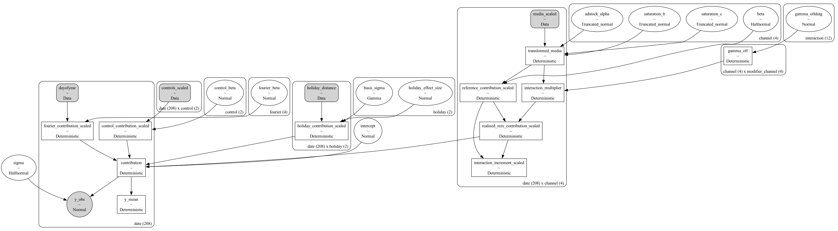
The full model graph makes the flow concrete: transformed media and the base coefficients form each channel’s reference contribution; the other channels enter through the directional \(\gamma\) matrix to form the multiplier; the realised-mix contributions are summed with controls, seasonality and holidays before the likelihood. It is wide, so click to zoom into any part.
The prior on the interaction, and its scale
A prior such as \(\gamma_{ij}\sim\mathcal N(0,\sigma_\gamma)\) cannot be interpreted without the scale of transformed media, because \(\gamma\) only ever enters multiplied by \(m_{j,t}\). With \(\sigma_\gamma=0.4\) and a single modifier near typical transformed-media levels, the implied prior on the multiplier \(M_{i,t}=\exp(\sum_j\gamma_{ij}m_{j,t})\) is fairly gentle. The issue is what happens when several modifiers are active at once: independent pairwise priors that look reasonable in isolation can imply a surprisingly wide prior over the total multiplier.
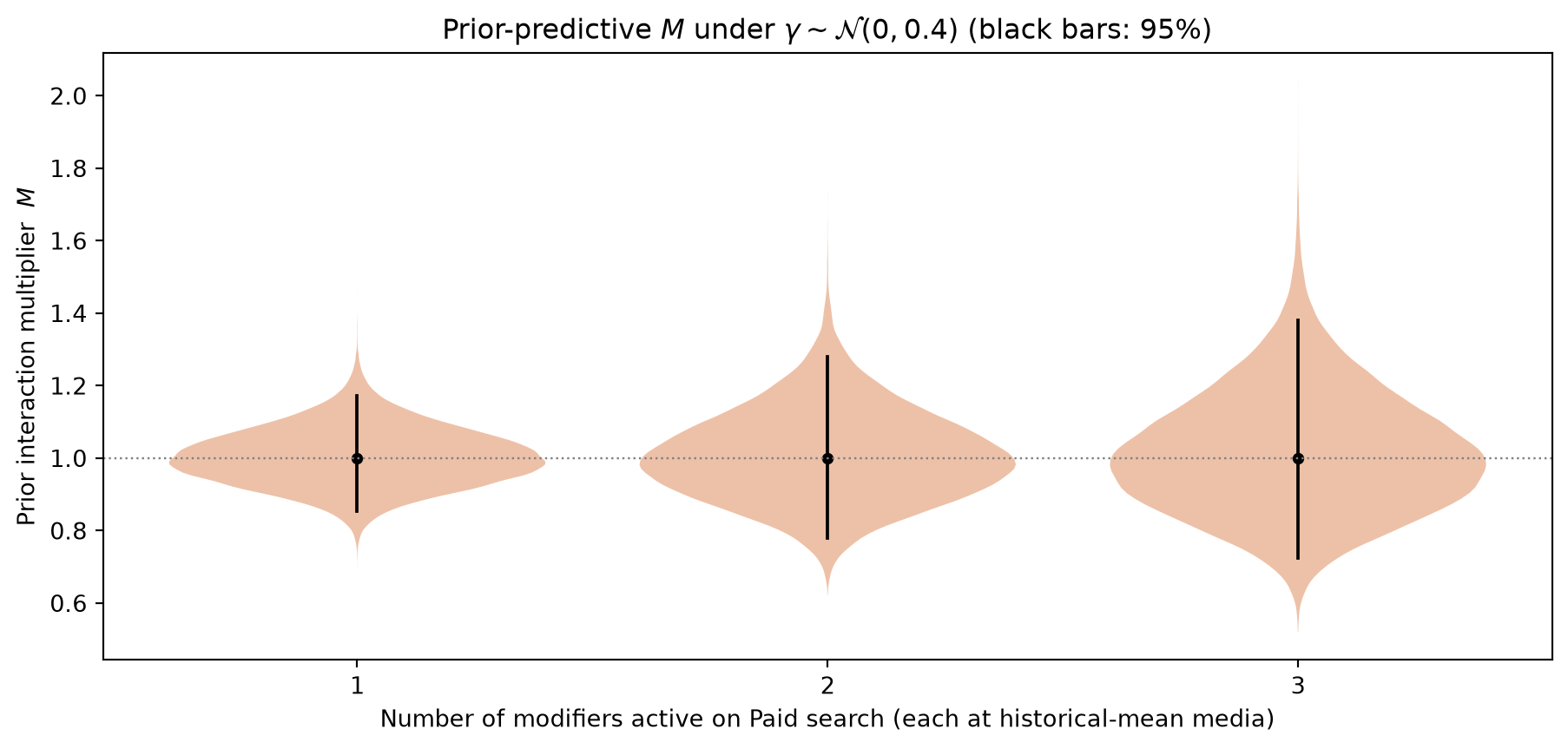
| Active modifiers | Prior 95% interval for M | |
|---|---|---|
| 0 | 1 | [0.85, 1.17] |
| 1 | 2 | [0.78, 1.28] |
| 2 | 3 | [0.72, 1.38] |
Even with a modest per-pair prior, three active modifiers admit roughly a \(\pm 30\%\) swing in effectiveness before any data are seen, which means the prior width, media scale and number of candidate modifiers must be considered together rather than one coefficient at a time.
What is the reference environment?
The multiplier above uses zero surrounding media as its reference, meaning \(M_{i,t}=1\) when \(m_{j,t}=0\) for all \(j\neq i\). Although this provides a clean synthetic anchor, it may sit far from where real data live because channels are rarely all dark at once. An alternative is to centre the interaction on the average historical environment:
\[ M_{i,t} = \exp\!\left(\sum_{j\neq i}\gamma_{ij}\left(m_{j,t}-\bar m_j\right)\right), \]
which defines the reference at the mean transformed-media environment and can reduce posterior dependence between the base effects and the interaction terms. I keep the zero-media reference here because it makes the decomposition and worked example transparent, but for real data the centred specification is an open modelling choice worth considering, since the interpretation of \(C^{\mathrm{ref}}\) depends on which reference is used.
Illustrating the reporting framework
To make the reporting concrete, I fit the model to a synthetic four-year, four-channel weekly dataset containing a small number of directional interactions. This keeps the outputs easy to interpret while demonstrating how an interaction-aware model changes contribution, ROAS and response-curve reporting; it does not establish that every cross-channel interaction can be reliably identified.
As with any MMM, the posterior estimates depend on the variation in the data, the media transformations, the controls and the priors. I return to the identification problem later; for now, the fitted example is used to illustrate the reporting framework. I report posterior point summaries alongside 94% highest-density intervals (HDIs) where appropriate, and every derived quantity is formed draw by draw before summarising.
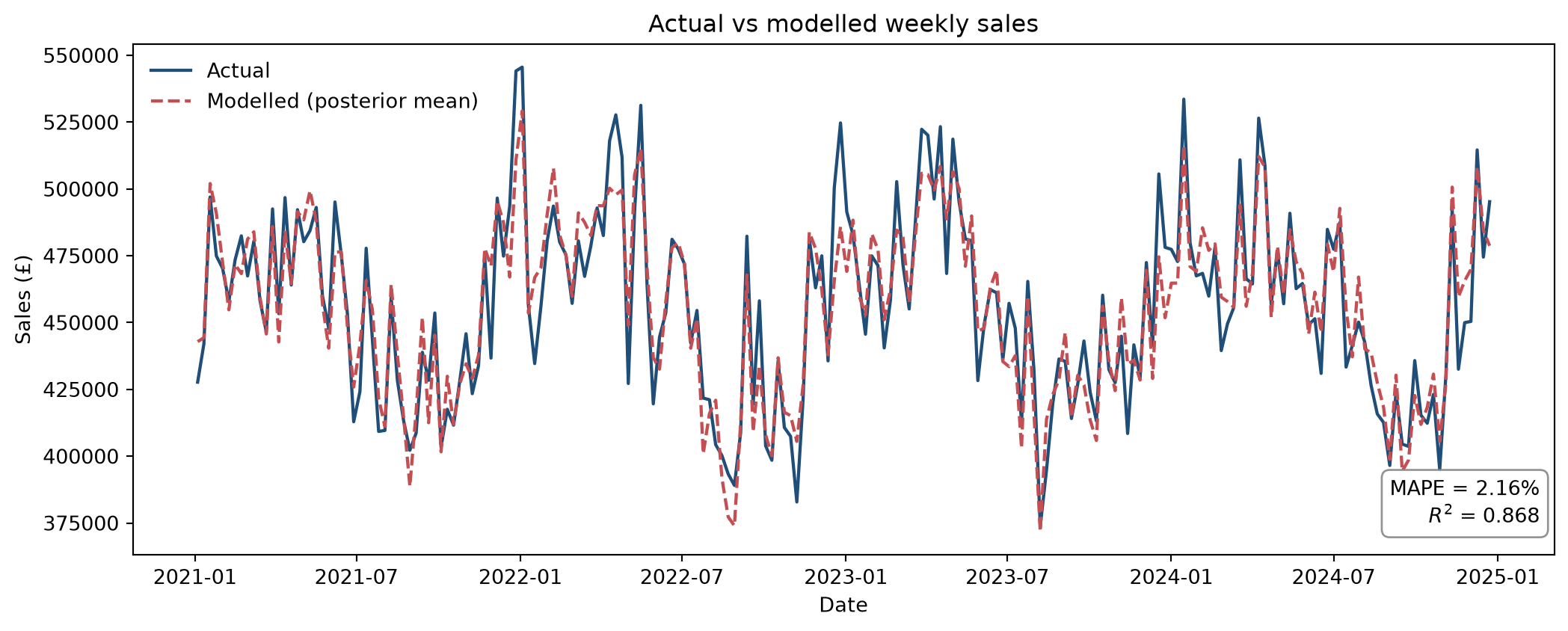
The posterior predictive distribution broadly tracks the synthetic outcome and provides a fitted example for examining contribution and response reporting, although predictive fit alone cannot establish that the individual base and interaction effects are uniquely identified.
Reference vs realised-mix contribution
The decomposition reports, per channel, the reference contribution, the interaction increment and the realised-mix contribution. Because the increment is formed draw by draw, the arithmetic reconciles: realised-mix = reference + increment.
| Channel | Reference contribution | Interaction increment | Realised-mix contribution | Realised-mix 94% HDI | Realised-mix share | |
|---|---|---|---|---|---|---|
| 0 | Paid search | £2.95m | £0.18m | £3.13m | [2.11, 4.34]m | 26.6% |
| 1 | Online video | £2.12m | £0.27m | £2.39m | [1.51, 3.44]m | 20.4% |
| 2 | Paid social | £3.26m | £0.04m | £3.30m | [2.21, 4.38]m | 27.9% |
| 3 | Display | £2.84m | £0.06m | £2.90m | [1.81, 4.05]m | 24.5% |
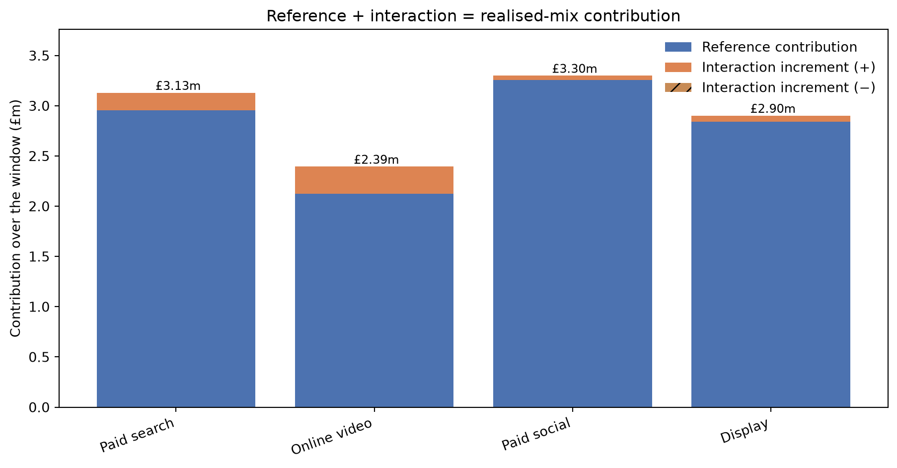
Because the estimated interactions are modest, realised-mix contributions sit close to their references, with the largest increment attaching to Paid search, which is the channel the model most associates with a video uplift.
ROAS under interactions
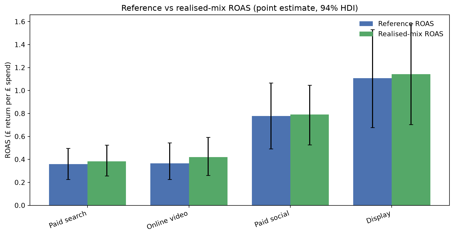
The same split carries into ROAS. Using raw spend \(x_{i,t}\) in the denominator (not transformed media):
\[ \text{Reference ROAS}_i = \frac{\sum_t C_{i,t}^{\mathrm{ref}}}{\sum_t x_{i,t}}, \qquad \text{Realised-mix ROAS}_i = \frac{\sum_t C_{i,t}^{\mathrm{mix}}}{\sum_t x_{i,t}}. \]
| Channel | Reference ROAS | Realised-mix ROAS | Interaction difference | |
|---|---|---|---|---|
| 0 | Paid search | 0.36 [0.23, 0.50] | 0.38 [0.26, 0.53] | +0.02 |
| 1 | Online video | 0.37 [0.23, 0.54] | 0.42 [0.26, 0.59] | +0.05 |
| 2 | Paid social | 0.78 [0.49, 1.07] | 0.79 [0.53, 1.05] | +0.01 |
| 3 | Display | 1.11 [0.68, 1.53] | 1.14 [0.70, 1.58] | +0.02 |
Directional interaction reporting
This formulation places the interaction increment inside the affected channel’s realised-mix contribution. That choice has a consequence worth stating plainly: under this convention the modifying channel does not receive direct channel-level credit for the value it creates elsewhere, so its reported contribution and ROAS may understate its wider role in the media system. The table below makes the directional relationships visible in their own right.
| Modifier (j) | Affected (i) | γ (median [94% HDI]) | Increment (£m) | |
|---|---|---|---|---|
| 0 | Online video | Paid search | +0.36 [-0.36, +1.12] | £+0.21m |
| 1 | Paid search | Online video | +0.35 [-0.37, +1.09] | £+0.21m |
| 2 | Display | Paid social | +0.17 [-0.43, +0.78] | £+0.15m |
| 3 | Paid search | Paid social | -0.09 [-0.71, +0.59] | £-0.08m |
| 4 | Paid social | Display | +0.10 [-0.54, +0.80] | £+0.07m |
| 5 | Display | Online video | +0.11 [-0.55, +0.77] | £+0.07m |
The contribution table answers “within which channel’s response does the increment appear?”, whereas this table answers “which channel modified which other channel?”. Because these are different questions, there is no single universal rule for allocating the value between them.
Response curves depend on the media mix
Once interactions are present, the model no longer implies a single unconditional response curve for a channel. It implies a family of response curves, conditional on the surrounding media environment. The figure below shows Paid search under three environments. Each curve is a steady-state curve: it answers “if the channel spent a constant amount every week until its adstock settled, what weekly contribution would the model imply?”, with modifier channels likewise held at a constant weekly spend until steady state. The x-axis stays within the historically observed range.
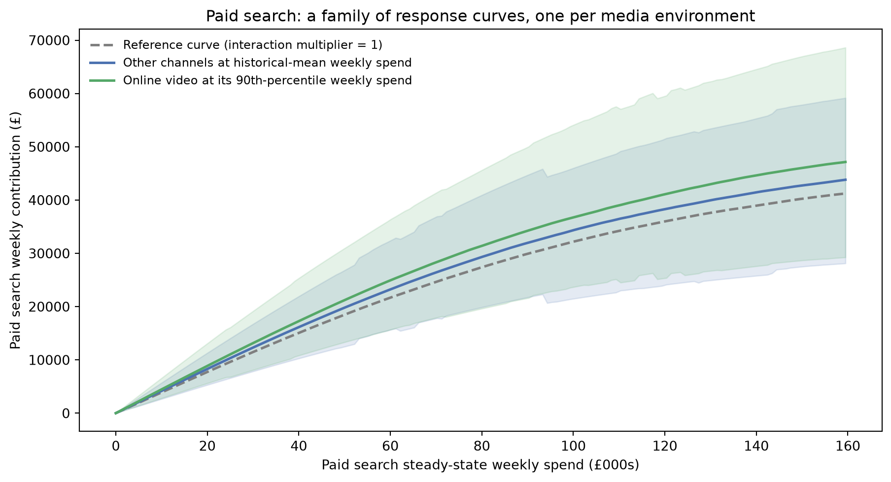
The gap between the curves shows the interaction at work, with the same steady-state search spend earning more when video runs alongside it.
What makes this difficult in practice
Writing the interaction model is straightforward, but determining whether the data can distinguish the effects it contains is much harder.
- Identification. If channels launch, pause and scale together, as they often do in an integrated campaign, there is little independent variation to separate a channel’s direct effect, its cross-channel effect, campaign timing and demand. When channels share similar timing and spend patterns, the model can trade off a channel’s base effect against the interaction term, allowing overall prediction to remain strong even when the separate components are weakly identified.
- Correlation and priors are separate problems. With limited data, priors can materially influence the posterior (Jin et al. 2017). Strong correlation between channels is an additional identification problem: several explanations can fit the same movement in the outcome, so a non-zero \(\gamma_{ij}\) may equally reflect omitted demand, common timing or a misspecified transform.
- Coefficient size is not commercial impact. A large \(\gamma_{ij}\) does not necessarily imply a large interaction increment. The commercial effect also depends on the affected channel’s base effectiveness \(\beta_i\), the transformed activity \(m_{i,t}\) and \(m_{j,t}\), and how much the channels overlap through time.
- Experiments help most. Staggered campaigns, geo variation and holdouts provide better identifying information than observational time series; partial pooling across geographies can also help (Sun et al. 2017). None of this manufactures evidence the data do not contain.
How many interaction parameters?
There is also a plain counting problem. For \(N\) channels, a fully directional pairwise model has \(N(N-1)\) off-diagonal interaction coefficients, on top of everything the model already carries (base coefficients, adstock, saturation, seasonality, controls, noise).
| Channels \(N\) | Directional interactions \(N(N-1)\) | Symmetric \(N(N-1)/2\) |
|---|---|---|
| 4 | 12 | 6 |
| 8 | 56 | 28 |
| 12 | 132 | 66 |
| 20 | 380 | 190 |
These parameters can be expressed in PyMC, but computational feasibility is not the same as statistical identification, and the two should not be confused. As the interaction set grows, the parameter count rises, the posterior geometry becomes harder to sample, weak identification spreads mass across trade-offs between base and interaction terms, and the interpretation burden grows faster still. Clean convergence diagnostics would tell me the sampler explored the posterior; they would not tell me the interaction parameters are identified. With 20 channels and 380 interactions, I would struggle to defend most of those numbers to a stakeholder.
How many response curves?
Reporting suffers from a second kind of explosion. Under a simplified binary view where each of the other \(N-1\) channels is either “active” or “inactive” in a focal channel’s environment, the number of environments is
\[ \sum_{k=0}^{N-1}\binom{N-1}{k} = 2^{\,N-1}, \]
which follows from the binomial theorem with \(a=b=1\); across all \(N\) channels that is \(N\,2^{\,N-1}\). One focal channel already has \(2^{3}=8\) environments with four channels and \(2^{9}=512\) with ten. Because modifier levels are continuous rather than binary, the full model technically implies an infinite family of conditional response curves, so practical reporting requires fixing an environment of interest, as in the figure above, or exploring the results interactively. This is another reason to keep the interaction set small.
A targeted approach is more defensible
My current preference is therefore to estimate a small number of deliberately chosen interactions rather than every possible relationship. Instead of fitting the full off-diagonal matrix, restrict attention to a set of pairs
\[ \mathcal{I} = \left\{ (i,j) : \text{there is a substantive reason to estimate } \gamma_{ij} \right\}, \]
and fit only those:
\[ C_{i,t}^{\mathrm{mix}} = \beta_i\, m_{i,t}\, \exp\!\left( \sum_{j:\,(i,j)\in\mathcal{I}} \gamma_{ij}\, m_{j,t} \right). \]
A “substantive reason” means a clear strategic relationship, a known customer journey, a demand-creating channel feeding a demand-capturing one, experimental or lift-study evidence, or repeated evidence across regions and campaigns. The hierarchical treatment in Naik and Peters (2009) provides a useful precedent for imposing substantive structure on a model containing several media interactions. And the display–search relationship estimated by Kireyev et al. (2016) illustrates why candidate interactions should be grounded in a plausible customer journey and evaluated in the specific context being modelled, rather than assumed everywhere.
Where this could go next
The natural next step is budget optimisation because, once a channel’s return depends on the whole mix, allocation stops being a set of independent per-channel curves and becomes a joint problem. Moving spend into video changes both video’s own contribution and search’s effectiveness, a topic that deserves its own treatment.
Conclusion
Explicit cross-channel modelling is possible and potentially valuable, particularly where there is a clear reason to believe one channel changes the effectiveness of another. The framework here gives a concrete, reconciled way to report it: a reference contribution, an interaction increment and a realised-mix contribution that add up, with the matching ROAS and response-curve consequences.
The approach is also complex and depends on both its assumptions and the variation present in the data. Estimating every possible relationship inflates the parameter count, identification demands and reporting burden, so the method is best used selectively. Where strategic, experimental or empirical evidence supports a particular interaction, explicitly estimating it may provide a richer model-based account of the relationship between those channels; where that evidence is absent, an all-channel interaction model is likely to introduce more uncertainty than useful information.
References
Jin, Yuxue, Yueqing Wang, Yunting Sun, David Chan, and Jim Koehler. 2017. Bayesian Methods for Media Mix Modeling with Carryover and Shape Effects. Google Inc.
Kireyev, Pavel, Koen Pauwels, and Sunil Gupta. 2016. “Do Display Ads Influence Search? Attribution and Dynamics in Online Advertising.” International Journal of Research in Marketing 33 (3): 475–90. https://doi.org/10.1016/j.ijresmar.2015.09.007.
Naik, Prasad A., and Kay Peters. 2009. “A Hierarchical Marketing Communications Model of Online and Offline Media Synergies.” Journal of Interactive Marketing 23 (4): 288–99. https://doi.org/10.1016/j.intmar.2009.07.005.
Naik, Prasad A., and Kalyan Raman. 2003. “Understanding the Impact of Synergy in Multimedia Communications.” Journal of Marketing Research 40 (4): 375–88. https://doi.org/10.1509/jmkr.40.4.375.19385.
Naik, Prasad A., Kalyan Raman, and Russell S. Winer. 2005. “Planning Marketing-Mix Strategies in the Presence of Interaction Effects.” Marketing Science 24 (1): 25–34. https://doi.org/10.1287/mksc.1040.0083.
Sun, Yunting, Yueqing Wang, Yuxue Jin, David Chan, and Jim Koehler. 2017. Geo-Level Bayesian Hierarchical Media Mix Modeling. Google Inc.