Reach & Frequency Modelling: A deep dive into modelling reach
How audience breadth and repeat exposure shape media response, and why the reach assumption matters for planning
In many media mix models (MMMs), media activity is represented by an exposure measure such as impressions. This captures how much advertising was delivered. Reach and frequency add a view of how those impressions were distributed across people.
Reach is the number of unique people who see an ad in a modelled region and period. Average frequency is the average number of times a reached person is exposed to an ad in that period. Together, they account for delivery:
When reliable reach data and enough variation are available, modelling reach and frequency lets an MMM learn about the campaign setup: was that delivery spread across more people, or repeated among fewer? Impressions alone are still a sensible input when the extra data are unavailable or the delivery mix barely changes. Compare two plans in the same market and period, each with 400,000 impressions:
One impression total, two delivery patterns
People count shows reach. Their colour shows average frequency.
Plan A Broader reach
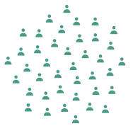
200,000 people reached · 2 exposures on average
200,000 × 2 = 400,000 impressions
Plan B Repeated exposure
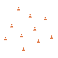
50,000 people reached · 8 exposures on average
50,000 × 8 = 400,000 impressions
If later exposures have a different effect from earlier ones, these plans can have different modelled responses despite the equal impression count. The difference can help a team discuss audience expansion and repetition, alongside creative and audience quality.
This requires more granular delivery data, not merely another column of spend. For each channel, geo and period, use unique reach in that period and average frequency equal to impressions divided by that reach. Cumulative campaign reach is a different measure. If campaign-level splits matter, retain campaign-level delivery records and model them separately only where the outcome data and variation support that detail; otherwise deduplicate reach before aggregating to the model’s channel, geo and period. Google Meridian is one example of a reach-and-frequency specification; its data guidance makes the same geographic and time-grain requirement.
How the model combines reach and frequency
A reach-and-frequency model can let each additional exposure add less response as frequency rises, multiply that frequency response by the number of people reached, and carry some effect into later periods:
Here β sets the response scale. Saturation lets later exposures add less than earlier ones; it does not imply that extra exposures are harmful. Adstock lets some response persist into later periods. Notice that reach enters as a simple multiplier. At a fixed frequency, doubling reach doubles this part of the modelled response. That assumption becomes important when projecting a campaign designed to reach a broader audience.
Meridian’s published specification provides one version of this structure. The response curves below isolate the reach-and-frequency response before carryover, so they do not depend on a chosen time window. They show illustrative units from a synthetic example, not measured campaign lift or a recommended frequency target.
To isolate delivery, the two plans use the same frequency-response parameters and response scale. At 400,000 impressions, plan A’s 200,000 reach and frequency two produce 13.7 illustrative response units; plan B’s 50,000 reach and frequency eight produce 9.4. The curves differ because the plans allocate impressions between broader reach and repeated exposure differently. The result is not evidence that one real channel is intrinsically stronger.
Same impressions, different delivery
Move either plan's average frequency. Both coloured points stay at 400,000 impressions, so higher frequency means lower reach. Both curves use the same model parameters; they differ because one delivery plan reaches more people while the other repeats exposure.
Interactive controls require JavaScript. The static chart below shows the default comparison.
Swipe or scroll sideways to see the full chart.
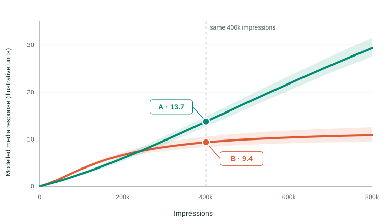
For this illustration, average frequency rises linearly from one as impressions grow, while reach equals impressions divided by frequency. Those delivery paths allocate additional impressions differently between new people and repeat exposures. Plan B’s response flattens sooner as frequency saturates and reach grows slowly; A keeps reaching more people. The shaded bands show parameter variation within the illustrative model, not evidence of either plan’s real-world lift.
Projecting broader reach with a linear response
Linear reach assumes that every additional person reached adds the same expected response, at a fixed frequency and with the other model terms held constant. If 100,000 people at frequency four produce 10 response units, the model projects 20 units at 200,000 people and 30 at 300,000. There is no bend in the reach response to signal that the next audience might be less valuable.
For example, consider specialist payroll software sold only to large employers. A campaign reaches 100,000 relevant decision makers at frequency four. A broader campaign could double reach by adding 100,000 people who have little influence over payroll purchases. Linear reach would still project twice the contribution, even though the new audience may generate very little extra demand.
This can create three problems when using the model to plan:
- Audience quality is assumed to stay constant. A unique person counts equally in the reach term whether they are a likely buyer or outside the eligible audience.
- Expansion can look more attractive than it is. If acquisition costs are held constant too, the model keeps assigning the same return to additional reach. That can steer budget towards broadening the audience instead of another channel, creative or targeting strategy.
- The forecast can outrun the evidence. A model fitted on narrower campaigns may carry the same slope far beyond the reach levels and audience mix it has observed.
Meridian’s optimisation guide shows how reach scales with budget at a fixed frequency. The business question is whether the next people reached should receive the same response weight. Where that is doubtful, consider a different response–reach relationship and check whether it changes the recommendation.
Linear reach is often a fair approximation over the range of activity the business actually uses. It also avoids extra parameters that can be difficult to estimate; Google’s reach modelling guidance discusses this trade-off. The point is to test a consequential assumption, rather than replace linear reach automatically.
How might the value of additional reach change?
Frequency saturation and reach saturation describe different mechanisms. The former says a person’s later exposures may add less than their earlier ones. The latter says the next new person reached may be less responsive than earlier reached people.
To test how much the reach assumption matters, we can change just that part of the model and compare the resulting forecasts and decisions. This is a sensitivity analysis: asking whether the recommendation still holds under another plausible assumption. Here we replace raw reach with an effective-reach function \(G(r)\), while keeping frequency saturation, carryover and the response scale unchanged.
The examples below share the same initial slope. The solid line in each panel is its proposed effective-reach response; the dashed line is the linear baseline. The parameters are illustrative choices, not fitted estimates. \(G(r)\) measures effective reach as a function of observed reach \(r\); the actual count of unique people does not change.
Linear reach
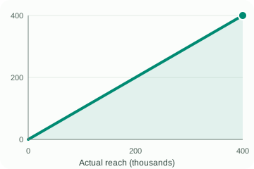
\(G(r)=r\). Each new person adds the same expected effect at a fixed frequency. This is the baseline assumption.
Gradual decline
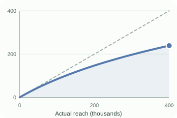
\(G(r)=K\log(1+r/K)\). The next audience is gradually less responsive, but further reach still adds value.
Faster saturation
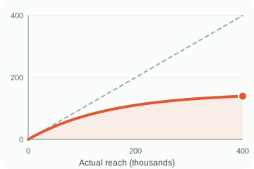
\(G(r)=K(1-e^{-r/K})\). An eligible or attentive audience becomes harder to find more quickly.
Eligible-audience cap
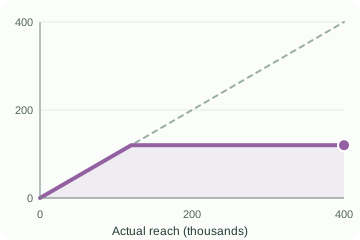
\(G(r)=\min(r,R_{\mathrm{eligible}})\). Beyond a defensible eligible-audience limit, more reach adds no modelled value.
The visuals use \(K=250{,}000\) for gradual decline, \(K=150{,}000\) for faster saturation, and \(R_{\mathrm{eligible}}=120{,}000\) for the cap. Here \(K\) is an illustrative reach scale. These are not competing fitted models. Audience composition, cross-channel overlap and repeat exposure across weeks can also produce apparently diminishing value; a curve alone cannot identify which mechanism is operating. If qualified and broad audiences can be measured separately, segmenting them may express the business question more directly.
How would a non-linear reach function affect decision making?
Suppose we have fitted our MMM and one channel typically reaches 100,000 people at an average frequency of four in a geo and period: 400,000 impressions. We now want to plan the next campaign. Should we reach more people, repeat exposure more often, or do a little of both?
The surface below lets us explore that question. Each point is a reach × frequency combination; its height is the modelled contribution before carryover. The dark dot marks the current setup. Use the dropdown to compare the reach assumptions, starting with linear reach and then faster saturation. We keep the frequency-response parameters and coefficient the same, so any difference comes from the reach assumption. These are illustrative scenarios, not separately fitted models.
Explore reach, frequency and contribution
Choose a reach function, then use the buttons to rotate the same surface to a preset view and highlight a slice. Scrolling over the graphic moves the page.
The dropdown and slice buttons need JavaScript. The illustration and comparison table below show the default scenarios.
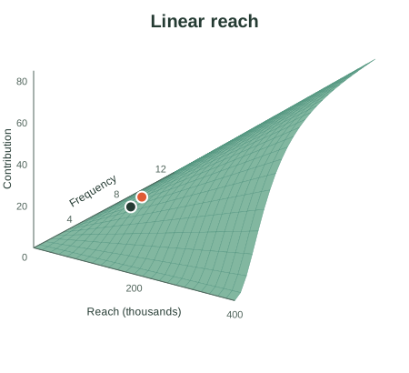
Use the view buttons to turn the surface; hover over a grid cell for approximate values.
How to read the surface and its slices:
- Select response × reach slice to rotate the surface towards the reach axis. The highlighted cut holds frequency at four. The complete surface stays visible behind it, with the same axis ranges. Only audience breadth changes along the highlighted curve. A straight line keeps rewarding each extra person equally; a bending line assigns less to the next person.
- Select response × frequency slice to see a cut at 100,000 reach. The same surface rotates towards the frequency axis and highlights that cut. Repetition initially builds response, then adds progressively less. The same frequency function is used in every scenario, although its contribution scale changes with effective reach. The view buttons change the angle, not the contribution scale.
- Return to the full surface to see both together. A steep part of the surface means more response from a small change in delivery. A flatter part means less additional response. Hover over a grid cell for approximate reach, frequency and contribution.
Where does the surface start to flatten?
The orange dot is an illustrative knee, used here as a reference for the approach to the plateau. We locate it in the separate reach and frequency slices where their falling gradients are closest to the slope of \(y=x\). First, each slice’s horizontal and vertical ranges are scaled to 0–1; otherwise changing reach from people to thousands would change the answer. The fixed comparison ranges are 0–400,000 reach and 1–12 average exposures. For the hard cap, we mark the corner where the slope drops to zero.
| Reach assumption | Reach at the knee | Frequency at the knee |
|---|---|---|
| Linear reach | No distinct reach knee | About 4.9 |
| Gradual decline | About 169,000 | About 4.9 |
| Faster saturation | About 158,000 | About 4.9 |
| Eligible-audience cap | 120,000 (the corner) | About 4.9 |
Notice how the candidate reach × frequency setting changes with the assumed reach response. Under faster saturation, about 158,000 reach × 4.9 frequency is a useful starting point for a planning recommendation to evaluate: beyond that knee the incremental gains become progressively smaller. With the cap, the corresponding reference is 120,000 × 4.9. Frequency stays the same here because we deliberately hold its response function constant. Linear reach has no distinct reach knee, so its orange dot marks only the frequency knee at the current 100,000 reach. Gradual decline has a knee over the chosen range but no finite ceiling.
These dots are planning references, not proven optimal settings or the exact onset of diminishing returns. Diminishing returns can begin before the knee, and the knee depends on the comparison range. Moving to either reference also changes the impression requirement. A recommendation needs to compare the extra contribution with cost, available audience and alternative uses of the budget.
Compare linear reach with faster saturation. Under linear reach, increasing reach from 100,000 to 200,000 at frequency four doubles contribution. Under the saturating function, the same move adds only about 51%; moving from 200,000 to 300,000 adds about 17%. There is no longer a clear instruction to keep increasing reach in the market or geo: the next audience may add too little response to justify its cost. Repetition, targeting, creative and other channels become part of the decision too.
Greater flexibility has a cost. A non-linear reach response can introduce one or two extra parameters to estimate per channel, depending on the function. Each smooth alternative shown here adds one reach-scale parameter \(K\); the cap adds an eligible-audience limit. If these are fixed from business evidence, they are scenario assumptions. If estimated, the model needs enough independent reach variation to distinguish them from the channel coefficient, frequency saturation and other effects. Weak data can leave several explanations equally plausible. Use business knowledge, defensible priors and validation to decide whether the additional flexibility is justified.
Key takeaways
- Impressions are a great metric to use in MMM. They measure delivered exposure and remain a useful input when reliable reach and frequency data are unavailable, or when the delivery mix does not vary enough to estimate separate effects.
- Reach and frequency add useful planning detail. They distinguish spreading impressions across more people from repeating exposure among fewer, connecting modelled contribution to decisions about audience breadth and repetition.
- Linear reach is often a fair assumption. It is simple and can work well within the observed range. Be cautious when a recommendation relies on reaching people beyond the audience that informed the model.
- Check whether the recommendation survives another plausible reach assumption. Run sensitivity analysis: change the reach response, compare the recommended settings, and assess whether the decision changes enough to matter. A more complicated curve is useful only if the evidence supports it.
- Have the business conversation. As an MMM vendor, discuss who the additional audience would be, how qualified they are, what they cost to reach and how much extrapolation the recommendation involves. Agree which assumptions are defensible before turning a surface or knee into a media plan.
JTP Analytics supports marketing mix modelling and model validation, including the assumptions that connect measurement to planning.